It is evident that the primes are randomly distributed but, unfortunately, we don’t know what ‘random’ means.
~R. C. Vaughan
The Problem we are interested
Here’s an age-old question consider a sequence of prime numbers \(2,3,5,7,11,13,17, \ldots\) Now given a prime number of \(P\) how would one predict the next prime number in the sequence?
This question is quite critical to deal with. But just because this question is a little bit critical, it does not stop us from exploring the various things about distribution primes. Prime numbers are one of the simplest yet most complicated and confusing topics in mathematics.
Euclid Theorem
Let’s start from the basics in middle school we learned that any number can be factored into prime numbers. For example, 30 can be written as \(30=3 \times2 \times5\) . So, we have two types of numbers primes and composite numbers. Euclid’s theorem is fairly straightforward. It states that
“There are an infinite number of primes.”
Let’s quickly go over a proof. This proof is actually pretty interesting. We have used proof by contradiction. We have assumed that this statement is false i.e., there are finite number of primes.
Let P be the product of every single prime number.
Let Q = P + 1
a) If Q is prime, then contradiction.
b) If Q isn’t prime then one of its prime factors p
Let’s look at one of those prime factors \(p\) and since \(p\) also divides \(P\), it should divides \(P-Q\) which is equal to \(1\) and since no prime number divides \(1\), it’s another contradiction. So it’s proved that ‘there are infinite number of prime’.
The Euler Product Formula
The Euler’s product formula generally defined as \(\displaystyle \sum_{n} \frac{1}{n^s} = \prod_{p} \frac {1} {1-p^{-s}}\) . Before going to discuss this, let’s understand the concept of series.
Series
A series can be highly generalized as the sum of all the terms in a sequence. However, there has to be a definite relationship between all the terms of the sequence. If think a bit deeper it’s actually cumulative sum of a given sequence of the terms. It’s obvious a series can be finite or infinite.
\[\sum_{i=1}^{n} i = \dfrac{n(n+1)}{2}\;\; \text{is a finite series}\] \[\sum_{n=0}^{\infty} r^n = 1+r+r^2+r^3+\ldots+r^n+ \ldots \;\; \text{is an infinite series}\]
Now let’s talk about harmonic series which we write as, \[\sum_{n=1}^{\infty} \dfrac{1}{n} = 1+\dfrac{1}{2}+\dfrac{1}{3}+\dfrac{1}{4}+ \ldots\]This series was shown divergent in \(14^{\text{th}}\) century. It means that it does not approach to a finite value. It just goes on to infinity. A harmonic series is a \(p\text{-series}\) which is a more general term. The general term of a \(p\text{-series}\) is as follows,
\[ \sum_{n=1}^{\infty}\dfrac{1}{n^{p}} = 1+\dfrac{1}{2^p}+\dfrac{1}{3^p}+\dfrac{1}{4^p}+ \ldots \]
The p-series will always converge when \(p>1\) . So converge means it approach to a finite value. Now we’ll define something call the zeta function which is written as follows,
\[ \zeta(s) = \sum_{n=1}^{\infty} \dfrac{1}{n^s} \]
Essentially, the zeta function gives the \(p\text{-series}\) given a value of \(p\). But how does this have anything to do with prime numbers? that’s why we talked about Euler’s product formula. Instead of just only giving the formula, I want to discuss the idea. So, let’s just start off with this zeta function.
\(\displaystyle \zeta(s) = \sum_{n=1}^{\infty} \dfrac{1}{n^s} = 1+\dfrac{1}{2^s}+\dfrac{1}{3^s}+\dfrac{1}{4^s}+\ldots \hspace{3cm} (1)\)
\(\implies \ \dfrac {1}{2^s}\zeta(s) = \dfrac{1}{2^s}+\dfrac{1}{4^s}+\dfrac{1}{6^s}+\dfrac {1}{8^s}+\ldots \; \; \text{[multiplying both sides by the second term of the sequence]} \hspace{2.5cm} (2)\)
So you can see the right side every single multiple of 2 in the denominator. So if we want to remove that from the original zeta function. So, next step we just subtract equation 2 from equation 1
\(\implies \left( 1-\dfrac{1}{2^s} \right) \zeta(s) = 1+\dfrac{1}{3^s}+\dfrac{1}{5^s}+\dfrac{1}{7^s}+\dfrac{1}{9^s}+\ldots \hspace{3cm} (3)\)
Then we’re going to repeat same process. So we’re gonna multiply both sides by the second term of the series now which is \(\dfrac{1}{3^s}\) if we do so we’ll have,
\(\implies \dfrac{1}{3^s}\left( 1-\dfrac{1}{2^s} \right)\zeta(s) = \dfrac{1}{3^s}+\dfrac{1}{9^s}+\dfrac{1}{15^s}+\dfrac{1}{21^s}+ \dfrac{1}{27^s}+\ldots \hspace{3cm} (4)\)
and we have these terms and then we subtract them from the equation 3 then we’ll have,
\(\implies \left(1-\dfrac{1}{3^s} \right) \left(1-\dfrac{1}{2^s} \right)\zeta(s) = 1+\dfrac{1}{5^s}+\dfrac{1}{7^s}+\dfrac{1}{11^s}+\dfrac{1}{11^s}+ \dfrac{1}{13^s}+\ldots\hspace{3cm} (5)\)
So, we do this process again and again you’ll see that every time we do this we are subtracting multiples of each number so the second term in our sequence is always going to prime and if we continue this process to infinity we will get something like this.
\[ \ldots \left(1-\dfrac{1}{11^s} \right) \left(1-\dfrac{1}{7^s} \right) \left(1-\dfrac{1}{5^s} \right) \left(1-\dfrac{1}{3^s} \right) \left(1-\dfrac{1}{2^s} \right)\zeta(s) = 1 \]
and if we move all the primes to the other side writing this formula we will have,
\[\sum_{\ n\in\mathbb{N} } \dfrac{1}{n^s} = \prod_{p\; \text{prime}} \frac {1} {1-p^{-s}} \] This is called the Euler’s product formula it gives us the first relation between zeta function and prime numbers and since this formula was discovered in 1737, modern study of prime numbers always based on the zeta function.
Prime Counting Function
The idea of the prime counting function is pretty simple. The prime counting function is the function \(\pi(x)\) giving the number of primes less than or equal to a given number \(x\). So, a few examples are,
\[\pi(5) \implies 3\]
\[\pi(10) \implies 4\] \[ \pi(20) \implies 8 \]
Basically, the prime counting function is a step function. It means that it’s not continuous. So, lets look at the graph of the prime counting function.
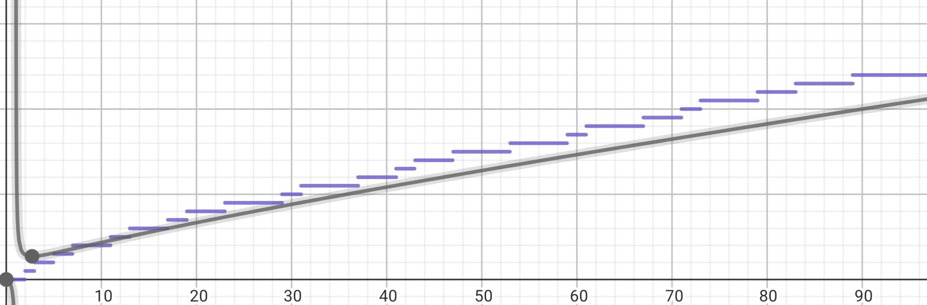
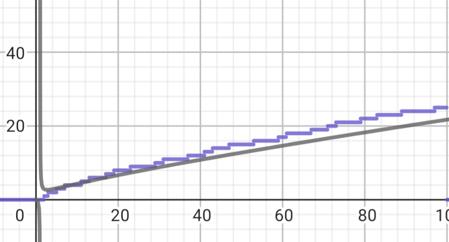
This function was introduced by Gauss in the 18th century and another thing Gauss showed was that you could approximate the value of the prime counting function with \(\frac{x}{ \ln(x)}\). This fact is called the prime number theorem. More formally,
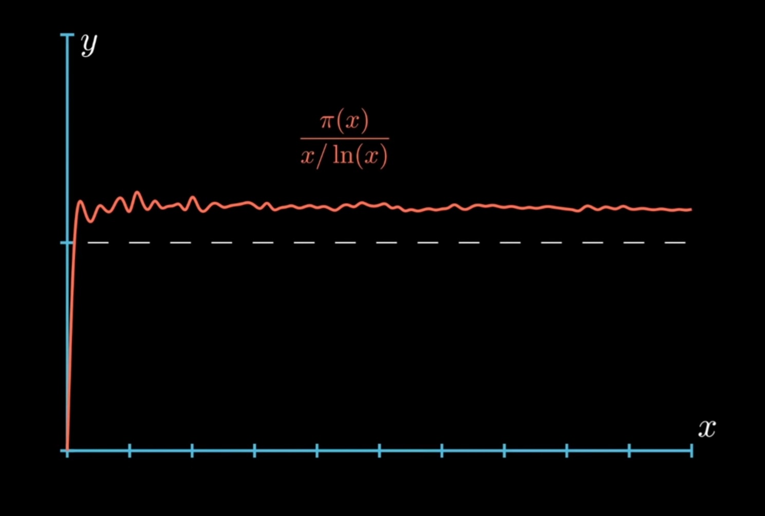
\[ \lim_{x \to \infty} \dfrac{\pi(x)}{\dfrac{x}{\ln(x)}} = 1 \]
If you take a look at this graph, you can see how it closely approaches 1 as \(x\rightarrow \infty\) .
Another result we can take from the prime number theorem i.e., the probability that a number chosen randomly from the set \(\{ 1,2,3, \ldots, x \}\) is roughly \(\frac{1}{\ln(x)}\). In terms of prime counting function the prime number theorem tells us that each average step in the prime counting function is around \(\ln(x)\). However there’s actually a better function to approximate the prime counting function.
Logarithmic Integral Function
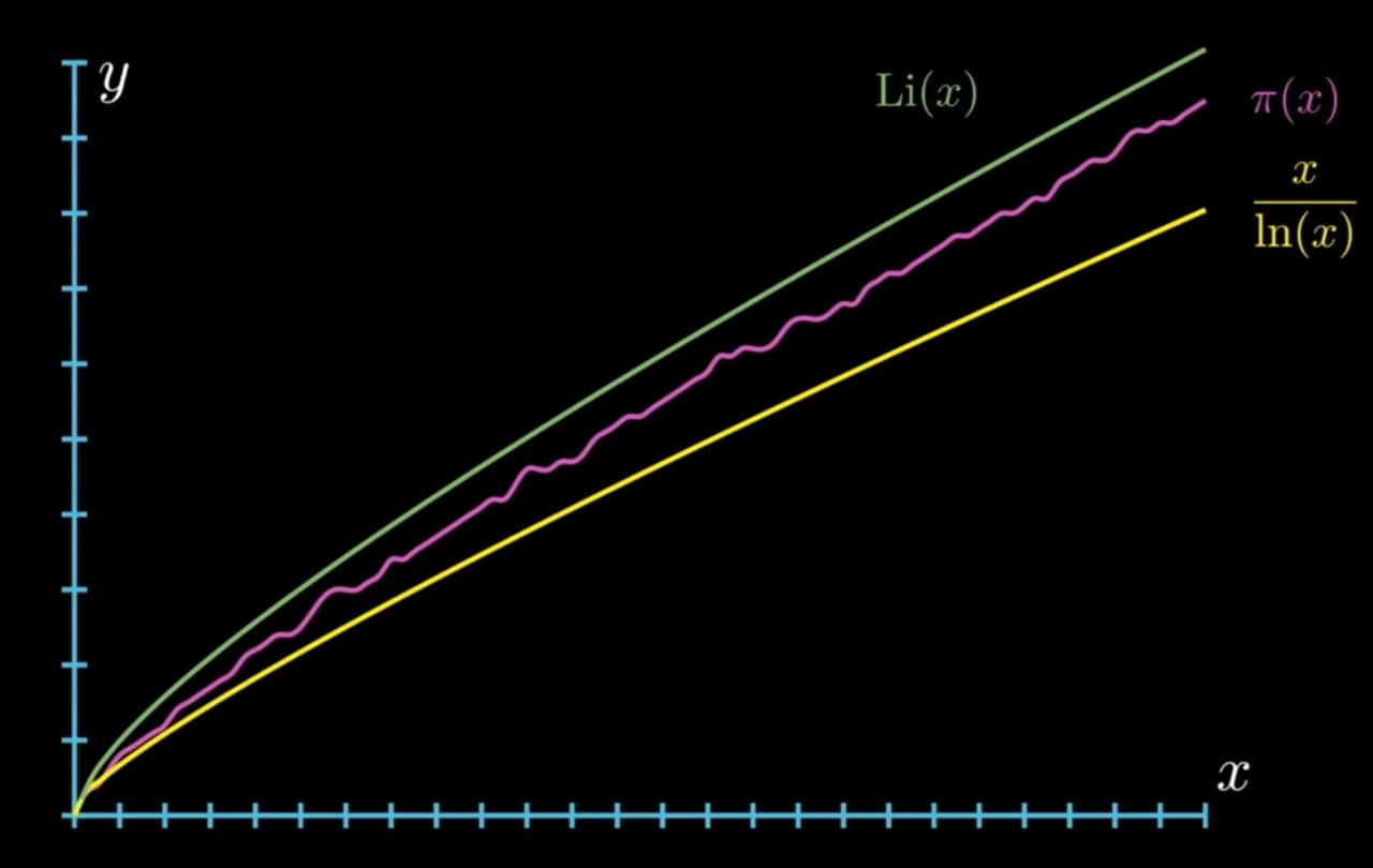
\[ \text{Li}(x) = \int_{2}^x \frac{dx}{\ln(x)} \]
It actually turns out that \(\text{Li}(x)\) is a better approximation for the prime counting function. Here you can look at all three of them graphed.
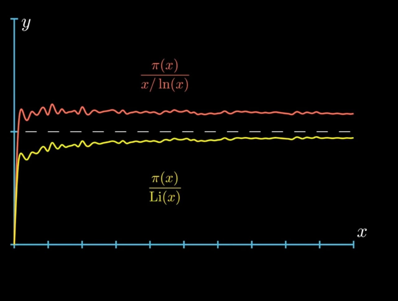
Since, \(\text{Li}(x)\) approximate \(\pi(x)\) then, \[\lim_{x \to \infty} \dfrac{\pi(x)}{\dfrac{x}{\ln(x)}} = 1 \]
This way of approximating the prime counting function by the logarithmic integral function is was discovered by Dirichlet after Gauss mailed him prime number theorem.
Riemann Zeta Function
Bernhard Riemann was a German mathematician who studied fields like mathematical analysis, differential geometry, and number theory. He was one of the first who studied what happens when you extend the domain of zeta function from a real to a complex number.
Riemann zeta function is essentially the zeta function that we have discussed earlier except we extend the domain to the whole complex plane and it converges for real component which is greater than 1.
Why This is True
Let’s look at some input,
\[\zeta\bigg(a+bi\bigg) = 1+ \bigg(\dfrac{1}{2}\bigg)^{a+bi}+\ldots \]Let’s focus on the first term and split it like this way \(\bigg(\dfrac{1}{2}\bigg)^{a+bi} = \bigg(\dfrac{1}{2}\bigg)^a \cdot \bigg(\dfrac{1}{2}\bigg)^{bi}\) . But what does it mean to take a complex exponent and what this turns out is that a complex exponential accounts for some rotation along the unit circle with no change in the magnitude.
What this means for us is that the magnitude of each term in the Riemann zeta function only depends on real component and so the Riemann zeta function converges for \(\text{Re}(z)>1\) . What about the other side of Riemann zeta function where real component is less than or equal to 1. So, Riemann used something called analytic continuation, basically he extended the domain of the zeta function by quote — unquote flipping it across. Riemann studied was the zeroes of the zeta function. To examine this let’s look at the formula of this Riemann zeta function with analytic continuation.
\[\zeta(s) = 2^s\pi^{s-1}\sin\bigg(\dfrac{\pi s}{2}\bigg)\Gamma(1-s)\zeta(1-s)\\
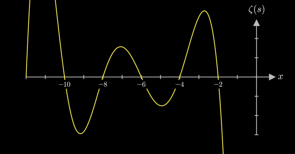
\zeta(s) = 0\;\; \text{when}\; \text{Re}(s) = -2n
\]
The term \(\Gamma(1-s)\) simply derive from the concept of the gamma function. Basically, the gamma function is to provide a continuous function that goes through a factorial point. Here, the sine term should equal to zero for all negative even integers. These zeros are called is trivial zeros for positive even integers the gamma function forms something called a pole which cancels out 0 of the sine function. A nice illustration of the trivial zeros of this Riemann zeta function would be real components of both the input and output. Look how \(\zeta(s) = 0\) at negative real numbers.
So, going back to the Euler product formula if the real component of the function is greater than 1 one of the products have to be equal zero for zeta to be equal to zero and this is impossible because of Euclid’s theorem which states that there are an infinite number of primes so the right component can not be equal to zero. That means the non-trivial zeros of the Riemann zeta function have have to have real component between 0 and 1. Let’s try to visualize them. The problem being that complex functions are like pretty hard to visualize. But this is our best we have showcase below.
We have fixed real component of input we’ve x-axis be the imaginary component. We have the graphs value of zeta vs imaginary part of zeta with real part 0.5. Notice that \(\text{Re}(s) = 0.5\) the real component intersect with the imaginary component at 0. This case lead us to a new concept which is the famous Riemann hypothesis. It states that all the non-trivial zeros of the Riemann zeta function have real component \(\frac{1}{2}\) or 0.5. Here this a spiral visualization of Riemann hypothesis which is given below.
Riemann and Primes
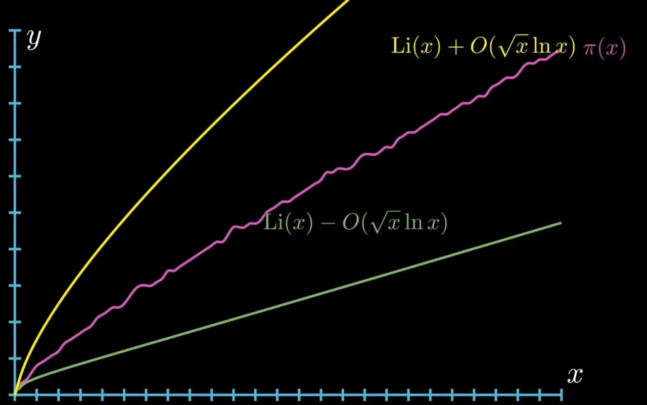
You’re wondering how all of this has any connection to the prime numbers. So, for this topic if we go back to the prime numbers theorem and recall how we could approximate the value of the prime counting function \(\pi(x)\) using the logarithmic integral function. The Riemann hypothesis helps us to talk about the error by which the logarithmic integral function can approximate this \(\pi(x)\) function. If the Riemann hypothesis is true this error is no more than some function of order \(\sqrt{x}\ \ln(x)\) and this goes both ways if you can prove that the error is a function of order \(\sqrt{x}\ \ln(x)\) the Riemann hypothesis is true.
A more direct question is how is the Riemann hypothesis and primes related?
\[ \pi(x) = \text{li}(x) - \sum_\rho \text{li}(x^\rho)-\log(2)+\int_{x}^\infty \dfrac{dt}{t(t^2-1)\log(t)} \]
So, this would be where we discuss about Riemann explicit formula. Riemann explicit formula gives us a direct formula for the prime counting function and the second term over here i.e., \(\displaystyle \sum_\rho \text{li}(x^\rho)\) is a sum of all non-trivial zeros of the Riemann-zeta function. There is a visualization attached below.
Here the graph is about Riemann’s explicit formula using the first 200 non-trivial zeros of the zeta function. And you can see how the graph becomes better and better approximation. Using non trivial zeros of the Riemann-zeta function you can approximate prime counting function to have a pretty high accuracy.
Conclusion
The Riemann hypothesis remains an unsolved problem in the field of number theory each year attempts are made and hopefully, we can see a concrete solution to this problem in the future.
References
Conrey, “The Riemann Hypothesis,” Notices of AMS, March, 2003, 341-353.
M. Agrawal, N. Kayal and N. Saxena, “Primes is in P” Annals of Math., 160,(2004), 781-793.
Visualizing the Riemann zeta function and analytic continuation.